Usage
SAS programs
Compute the quartiles of a randomly generated vector (with normal distribution) using default parameters of the quantile function:
DATA test;
	DO i = 1 TO 1000;
  		x = rand('NORMAL');
  		output;
	END;
	DROP i;
RUN;
%LET q_x=;
%quantile(x, idsn = test, _quantiles_ = q_x);
%PUT &q_x;
Do change the algorithm used for estimation:
%LET q_x=;
%quantile(x, type = 5, idsn = test, _quantiles_ = q_x);
%PUT &q_x;
Now compute the quintiles:
%LET q_x=;
%quantile(x, probs = 0.2 0.4 0.6 0.8, idsn = test, _quantiles_ = q_x);
%PUT &q_x;
Consider comparing the results obtained using both already existing PROC UNIVARIATE and the new implementation:
%LET probs = .2 .4 .6 .8;
%LET type = 8;
%quantile(x, probs=&probs, type=&type, method=DIRECT, _quantiles_ = q1);
%PUT &q1;

PROC UNIVARIATE DATA=test;
    VAR x;
    OUTPUT OUT=result PCTLPTS=&probs PCTLPRE=P_;
RUN;

DATA result;
    SET result;
    ARRAY P P_:;
    DO i=1 TO 5;
        CALL SYMPUT("q2","&q2 "!!LEFT(P(i)));
    END;
RUN;

%PUT &q2;
Python programs
Compute the quartiles of a randomly generated vector (with normal distribution) using default parameters of the quantile function:
>>> import numpy as np
>>> x = np.random.rand(1000)
>>> from quantile import quantile
>>> q = quantile(x)
>>> print(q)
	[0.10668975  0.19514584  0.33299627  0.53016722  0.89982259]
Do change the algorithm used for estimation:
>>> q = quantile(x, typ=5)
>>> print(q)
	[0.10668975  0.19323867  0.33299627  0.54542127  0.89982259]
Now compute the quintiles:
>>> q = quantile(x, probs=[0., .2, .4, .6, .8, 1.])
>>> print(q)
	[0.10668975  0.17672622  0.21760127  0.45610321  0.60035713  0.89982259]
Consider comparing the results obtained using both already existing scipy.mquantiles and the new implementation:
>>> probs = [0., .2, .4, .6, .8, 1.]
>>> typ = 8
>>> q1 = quantile(x, probs=probs, typ=typ, method='DIRECT')
>>> print(q1)
	[0.10668975  0.14370132  0.21388262  0.46239251  0.71022886  0.89982259]
>>> q2 = quantile(x, probs=probs, typ=typ, method='INHERIT')
>>> print(q2)
	[0.10668975  0.14370132  0.21388262  0.46239251  0.71022886  0.89982259]
It is possible to run (“call”) exactly the same estimations on an input file of sampled data, e.g.:
>>> ifile = "tests/sample1.csv"
>>> from io_quantile import IO_Quantile
>>> Q=IO_Quantile(probs=probs, typ=typ, method='DIRECT')
>>> q = Q(ifile)
>>> print(q)
	[-3.71390789 -0.84013745 -0.27581729  0.1972615   0.73643897  2.84320792]
An instance of the class IO_Quantile is associated to one possible configuration of the quantile estimation. Usually, you will define another instance to perform the estimation with different parameters, e.g. using specialised quantiles:
>>> probs = "V20"
>>> Q=IO_Quantile(probs=probs, typ=7)
>>> q = Q(ifile)
>>> print(q)
	[-1.77201688 -1.35332892 -1.02227673 -0.8369087  -0.65649296 -0.52217107
 	-0.40274654 -0.27525036 -0.17099489 -0.02049303  0.07102564  0.1971682
  	0.3350732   0.4536729   0.58860973  0.73606624  0.92265672  1.16084927
  	1.51058281]
But then it is possible to run the same estimation algorithm over different input files using that same, already defined, instance:
>>> ifile2 = "tests/sample2.csv"
>>> q2 = Q(ifile2)
>>> print(q2)
	[-1.50530344 -1.1758764  -0.97947549 -0.82893958 -0.67830867 -0.52803119
 	-0.38669867 -0.27675766 -0.15487459 -0.01350255  0.13391096  0.27587611
 	0.40033506  0.54753533  0.68432219  0.84362724  1.05800707  1.34756166
  	1.73445305]
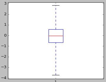
Note the definition of the IO_Quartile class that specifically runs estimation of quartiles, and also enables you to plot the associated boxplot:
>>> from matplotlib import pyplot
>>> from io_quantile import IO_Quartile
>>> Qu=IO_Quartile(typ=7);
>>> q = Qu(ifile)
>>> print(q)
	[-3.71390789 -0.65649296 -0.02049303  0.58860973  2.84320792]
>>> Qu.plot(ifile)
>>> pyplot.show()
R programs
Compute the quartiles of a randomly generated vector (with normal distribution) using default parameters of the quantile function:
> source("quantile.R")
> x <- rnorm(1000)
> quantile(x)
[1] -3.4336152 -0.6638305  0.0228467  0.7090099  3.1428912
Note the usage of names parameter for formatting the output vector (likewise the original stats::quantile function):
> quantile(x, names=TRUE)
        0%        25%        50%        75%       100%
-3.4336152 -0.6638305  0.0228467  0.7090099  3.1428912
Check that in INHERIT mode, we indeed wrap the original stats::quantile function:
> quantile(x, method='INHERIT')
        0%        25%        50%        75%       100%
-3.4336152 -0.6638305  0.0228467  0.7090099  3.1428912
> stats::quantile(x)
        0%        25%        50%        75%       100%
-3.4336152 -0.6638305  0.0228467  0.7090099  3.1428912
Do select other input parameters to test different types of implementation:
> quantile(x, type=5, probs=seq(0.,1.,0.1), names=TRUE)
        0%        10%        20%        30%        40%        50%        60%        70%        80%        90%       100%
-3.4336152 -1.3146826 -0.8156684 -0.5113350 -0.2285216  0.0228467  0.2787606  0.5420263  0.8906395  1.3397724  3.1428912
You can for instance check the effect of the choice of the estimation algorithm on the calculation of the median:
> quantile(x, type=1, probs=0.5, names=TRUE)
      50%
0.0198003
> quantile(x, type=3, probs=0.5, names=TRUE)
      50%
0.0198003
> quantile(x, type=5, probs=0.5, names=TRUE)
      50%
0.0228467
> stats::quantile(x, type=7, probs=0.5, names=TRUE)
      50%
0.0228467
> quantile(x, type=7, probs=0.5, names=TRUE)
      50%
0.0228467
> quantile(x, type=8, probs=0.5, names=TRUE)
      50%
0.0228467
> quantile(x, type=10, probs=0.5, names=TRUE)
      50%
0.0228467
Note that the method also works with data frame objects:
> d = data.frame(x=x)
> quantile(1, type=11, probs=0.5, names=TRUE, data=d)
      50%
0.0228467
Finally, you can, likewise the Python implementation, run the quantile estimation on an input file
> source("io_quantile.R")
> ifile = "/Users/gjacopo/Developments/quantile/tests/sample1.csv"
> io_quantile(ifile, names=TRUE)
         0%         25%         50%         75%        100%
-3.71390789 -0.65658941 -0.01801632  0.58892170  2.84320792