
import boto3
import configparser
import os
import urllib3

import folium
import geopandas as gpd
import rasterio
from rasterio.plot import show
import numpy as np
from matplotlib import pyplot

import tempfile
---------------------------------------------------------------------------
ModuleNotFoundError                       Traceback (most recent call last)
Cell In[1], line 1
----> 1 import boto3
      2 import configparser
      3 import os

ModuleNotFoundError: No module named 'boto3'
urllib3.disable_warnings()
Connection with S3 Bucket#
All Census GRID datasets are available on S3 Bucket. Below configuration allows to list and download defined datasets from there.
def s3_connection(credentials: dict) -> boto3.session.Session:
    """Establishes a connection to an S3 bucket.

    Args:
        credentials (dict): A dictionary containing AWS S3 credentials with keys
                            'host_base', 'access_key', and 'secret_key'.

    Returns:
        boto3.session.Session: A boto3 session client configured with the provided
                               credentials for interacting with the S3 service.
    """
    s3 = boto3.client('s3',
                      endpoint_url=credentials['host_base'],
                      aws_access_key_id=credentials['access_key'],
                      aws_secret_access_key=credentials['secret_key'],
                      use_ssl=True,
                      verify=False)
    return s3

# Load s3 credentials
config = configparser.ConfigParser()
config.read('/home/eouser/.s3cfg')
credentials = dict(config['default'].items())

# Connection with S3 eodata
s3 = s3_connection(credentials)
Browsing S3 bucket content#
response = s3.list_objects_v2(Bucket='ESTAT', Prefix='Census_GRID')
if 'Contents' in response:
    print("Objects in bucket:")
    # Iterate over each object
    for obj in response['Contents']:
        print(obj['Key'])
else:
    print("No objects found in the bucket.")
Objects in bucket:
Census_GRID/2021/ESTAT_Census_2021_V2.csv
Census_GRID/2021/ESTAT_Census_2021_V2.gpkg
Census_GRID/2021/ESTAT_Census_2021_V2.parquet
Census_GRID/2021/ESTAT_Census_2021_V2_SDMX_Metadata/CENSUS_INS21ES_A_AT_2021_0000.sdmx.xml
Census_GRID/2021/ESTAT_Census_2021_V2_SDMX_Metadata/CENSUS_INS21ES_A_BE_2021_0000.sdmx.xml
Census_GRID/2021/ESTAT_Census_2021_V2_SDMX_Metadata/CENSUS_INS21ES_A_BG_2021_0000.sdmx.xml
Census_GRID/2021/ESTAT_Census_2021_V2_SDMX_Metadata/CENSUS_INS21ES_A_CH_2021_0000.sdmx.xml
Census_GRID/2021/ESTAT_Census_2021_V2_SDMX_Metadata/CENSUS_INS21ES_A_CY_2021_0000.sdmx.xml
Census_GRID/2021/ESTAT_Census_2021_V2_SDMX_Metadata/CENSUS_INS21ES_A_CZ_2021_0000.sdmx.xml
Census_GRID/2021/ESTAT_Census_2021_V2_SDMX_Metadata/CENSUS_INS21ES_A_DE_2021_0000.sdmx.xml
Census_GRID/2021/ESTAT_Census_2021_V2_SDMX_Metadata/CENSUS_INS21ES_A_DK_2021_0000.sdmx.xml
Census_GRID/2021/ESTAT_Census_2021_V2_SDMX_Metadata/CENSUS_INS21ES_A_EE_2021_0000.sdmx.xml
Census_GRID/2021/ESTAT_Census_2021_V2_SDMX_Metadata/CENSUS_INS21ES_A_EL_2021_0000.sdmx.xml
Census_GRID/2021/ESTAT_Census_2021_V2_SDMX_Metadata/CENSUS_INS21ES_A_ES_2021_0000.sdmx.xml
Census_GRID/2021/ESTAT_Census_2021_V2_SDMX_Metadata/CENSUS_INS21ES_A_FI_2021_0000.sdmx.xml
Census_GRID/2021/ESTAT_Census_2021_V2_SDMX_Metadata/CENSUS_INS21ES_A_FR_2021_0000.sdmx.xml
Census_GRID/2021/ESTAT_Census_2021_V2_SDMX_Metadata/CENSUS_INS21ES_A_HR_2021_0000.sdmx.xml
Census_GRID/2021/ESTAT_Census_2021_V2_SDMX_Metadata/CENSUS_INS21ES_A_HU_2021_0000.sdmx.xml
Census_GRID/2021/ESTAT_Census_2021_V2_SDMX_Metadata/CENSUS_INS21ES_A_IE_2021_0000.sdmx.xml
Census_GRID/2021/ESTAT_Census_2021_V2_SDMX_Metadata/CENSUS_INS21ES_A_IT_2021_0000.sdmx.xml
Census_GRID/2021/ESTAT_Census_2021_V2_SDMX_Metadata/CENSUS_INS21ES_A_LI_2021_0000.sdmx.xml
Census_GRID/2021/ESTAT_Census_2021_V2_SDMX_Metadata/CENSUS_INS21ES_A_LT_2021_0000.sdmx.xml
Census_GRID/2021/ESTAT_Census_2021_V2_SDMX_Metadata/CENSUS_INS21ES_A_LU_2021_0000.sdmx.xml
Census_GRID/2021/ESTAT_Census_2021_V2_SDMX_Metadata/CENSUS_INS21ES_A_LV_2021_0000.sdmx.xml
Census_GRID/2021/ESTAT_Census_2021_V2_SDMX_Metadata/CENSUS_INS21ES_A_MT_2021_0000.sdmx.xml
Census_GRID/2021/ESTAT_Census_2021_V2_SDMX_Metadata/CENSUS_INS21ES_A_NL_2021_0000.sdmx.xml
Census_GRID/2021/ESTAT_Census_2021_V2_SDMX_Metadata/CENSUS_INS21ES_A_NO_2021_0000.sdmx.xml
Census_GRID/2021/ESTAT_Census_2021_V2_SDMX_Metadata/CENSUS_INS21ES_A_PL_2021_0000.sdmx.xml
Census_GRID/2021/ESTAT_Census_2021_V2_SDMX_Metadata/CENSUS_INS21ES_A_PT_2021_0000.sdmx.xml
Census_GRID/2021/ESTAT_Census_2021_V2_SDMX_Metadata/CENSUS_INS21ES_A_RO_2021_0000.sdmx.xml
Census_GRID/2021/ESTAT_Census_2021_V2_SDMX_Metadata/CENSUS_INS21ES_A_SE_2021_0000.sdmx.xml
Census_GRID/2021/ESTAT_Census_2021_V2_SDMX_Metadata/CENSUS_INS21ES_A_SI_2021_0000.sdmx.xml
Census_GRID/2021/ESTAT_Census_2021_V2_SDMX_Metadata/CENSUS_INS21ES_A_SK_2021_0000.sdmx.xml
Census_GRID/2021/ESTAT_OBS-VALUE-CHG_IN_2021_V2.tiff
Census_GRID/2021/ESTAT_OBS-VALUE-CHG_OUT_2021_V2.tiff
Census_GRID/2021/ESTAT_OBS-VALUE-CONFIDENTIAL_2021_V2.tiff
Census_GRID/2021/ESTAT_OBS-VALUE-EMP_2021_V2.tiff
Census_GRID/2021/ESTAT_OBS-VALUE-EU_OTH_2021_V2.tiff
Census_GRID/2021/ESTAT_OBS-VALUE-F_2021_V2.tiff
Census_GRID/2021/ESTAT_OBS-VALUE-LANDSURFACE_2021_V2.tiff
Census_GRID/2021/ESTAT_OBS-VALUE-M_2021_V2.tiff
Census_GRID/2021/ESTAT_OBS-VALUE-NAT_2021_V2.tiff
Census_GRID/2021/ESTAT_OBS-VALUE-OTH_2021_V2.tiff
Census_GRID/2021/ESTAT_OBS-VALUE-POPULATED_2021_V2.tiff
Census_GRID/2021/ESTAT_OBS-VALUE-SAME_2021_V2.tiff
Census_GRID/2021/ESTAT_OBS-VALUE-T_2021_V2.tiff
Census_GRID/2021/ESTAT_OBS-VALUE-Y_1564_2021_V2.tiff
Census_GRID/2021/ESTAT_OBS-VALUE-Y_GE65_2021_V2.tiff
Census_GRID/2021/ESTAT_OBS-VALUE-Y_LT15_2021_V2.tiff
Census_GRID/2021/read.me
Reading vector file to GeoDataFrame#
%%time

object_path = 'Census_GRID/2021/ESTAT_Census_2021_V2.gpkg'

# Create a temporary directory to store GeoPackage file
with tempfile.TemporaryDirectory() as tmpdirname:
    # Define local path to save GeoPackage file
    local_geopackage_path = os.path.join(tmpdirname, object_path.split('/')[-1])

    # Download the GeoPackage from S3
    s3.download_file('ESTAT', object_path, local_geopackage_path)

    # Read the GeoPackage into a GeoDataFrame
    gdf = gpd.read_file(local_geopackage_path)
CPU times: user 1min 6s, sys: 3.69 s, total: 1min 10s
Wall time: 1min 9s
# Geodata parameters
print(gdf.info())
print('----')
print(f'Coordinate system: {gdf.crs}')
<class 'geopandas.geodataframe.GeoDataFrame'>
RangeIndex: 4594018 entries, 0 to 4594017
Data columns (total 18 columns):
 #   Column              Dtype
---  ------              -----
 0   GRD_ID              object
 1   T                   int64
 2   M                   float64
 3   F                   float64
 4   Y_LT15              float64
 5   Y_1564              float64
 6   Y_GE65              float64
 7   EMP                 float64
 8   NAT                 float64
 9   EU_OTH              float64
 10  OTH                 float64
 11  SAME                float64
 12  CHG_IN              float64
 13  CHG_OUT             float64
 14  LAND_SURFACE        float64
 15  POPULATED           int64
 16  CONFIDENTIALSTATUS  float64
 17  geometry            geometry
dtypes: float64(14), geometry(1), int64(2), object(1)
memory usage: 630.9+ MB
None
----
Coordinate system: EPSG:3035
gdf.head()
| GRD_ID | T | M | F | Y_LT15 | Y_1564 | Y_GE65 | EMP | NAT | EU_OTH | OTH | SAME | CHG_IN | CHG_OUT | LAND_SURFACE | POPULATED | CONFIDENTIALSTATUS | geometry | |
|---|---|---|---|---|---|---|---|---|---|---|---|---|---|---|---|---|---|---|
| 0 | CRS3035RES1000mN1000000E1966000 | 259 | 143.0 | 116.0 | 38.0 | 190.0 | 29.0 | 86.0 | 113.0 | 94.0 | 47.0 | 220.0 | 24.0 | 11.0 | 0.6115 | 1 | NaN | POLYGON ((1966000 1000000, 1967000 1000000, 19... |
| 1 | CRS3035RES1000mN1000000E1967000 | 4 | 4.0 | 2.0 | 1.0 | 2.0 | 2.0 | 2.0 | 4.0 | 0.0 | 0.0 | 4.0 | 0.0 | 0.0 | 1.0000 | 1 | NaN | POLYGON ((1967000 1000000, 1968000 1000000, 19... |
| 2 | CRS3035RES1000mN1000000E1968000 | 0 | 0.0 | 0.0 | 0.0 | 0.0 | 0.0 | 0.0 | 0.0 | 0.0 | 0.0 | 0.0 | 0.0 | 0.0 | 1.0000 | 0 | NaN | POLYGON ((1968000 1000000, 1969000 1000000, 19... |
| 3 | CRS3035RES1000mN1000000E1969000 | 0 | 0.0 | 0.0 | 0.0 | 0.0 | 0.0 | 0.0 | 0.0 | 0.0 | 0.0 | 0.0 | 0.0 | 0.0 | 1.0000 | 0 | NaN | POLYGON ((1969000 1000000, 1970000 1000000, 19... |
| 4 | CRS3035RES1000mN1000000E1970000 | 0 | 0.0 | 0.0 | 0.0 | 0.0 | 0.0 | 0.0 | 0.0 | 0.0 | 0.0 | 0.0 | 0.0 | 0.0 | 1.0000 | 0 | NaN | POLYGON ((1970000 1000000, 1971000 1000000, 19... |
GeoDataFrame explanation#
GeoDataFrame inherits most of pandas DataFrame methods. That allows to work with GeoDataFrame on the same way.
# Creating new GeoDataFrame with defined columns
gdf[['GRD_ID','POPULATED','geometry']]
| GRD_ID | POPULATED | geometry | |
|---|---|---|---|
| 0 | CRS3035RES1000mN1000000E1966000 | 1 | POLYGON ((1966000 1000000, 1967000 1000000, 19... |
| 1 | CRS3035RES1000mN1000000E1967000 | 1 | POLYGON ((1967000 1000000, 1968000 1000000, 19... |
| 2 | CRS3035RES1000mN1000000E1968000 | 0 | POLYGON ((1968000 1000000, 1969000 1000000, 19... |
| 3 | CRS3035RES1000mN1000000E1969000 | 0 | POLYGON ((1969000 1000000, 1970000 1000000, 19... |
| 4 | CRS3035RES1000mN1000000E1970000 | 0 | POLYGON ((1970000 1000000, 1971000 1000000, 19... |
| ... | ... | ... | ... |
| 4594013 | CRS3035RES1000mN999000E1981000 | 1 | POLYGON ((1981000 999000, 1982000 999000, 1982... |
| 4594014 | CRS3035RES1000mN999000E1982000 | 1 | POLYGON ((1982000 999000, 1983000 999000, 1983... |
| 4594015 | CRS3035RES1000mN999000E1983000 | 0 | POLYGON ((1983000 999000, 1984000 999000, 1984... |
| 4594016 | CRS3035RES1000mN999000E1985000 | 0 | POLYGON ((1985000 999000, 1986000 999000, 1986... |
| 4594017 | CRS3035RES1000mN999000E1986000 | 0 | POLYGON ((1986000 999000, 1987000 999000, 1987... |
4594018 rows × 3 columns
# Filtering records based on attribute value
gdf[gdf['T']>20].head()
| GRD_ID | T | M | F | Y_LT15 | Y_1564 | Y_GE65 | EMP | NAT | EU_OTH | OTH | SAME | CHG_IN | CHG_OUT | LAND_SURFACE | POPULATED | CONFIDENTIALSTATUS | geometry | |
|---|---|---|---|---|---|---|---|---|---|---|---|---|---|---|---|---|---|---|
| 0 | CRS3035RES1000mN1000000E1966000 | 259 | 143.0 | 116.0 | 38.0 | 190.0 | 29.0 | 86.0 | 113.0 | 94.0 | 47.0 | 220.0 | 24.0 | 11.0 | 0.6115 | 1 | NaN | POLYGON ((1966000 1000000, 1967000 1000000, 19... |
| 14 | CRS3035RES1000mN1000000E1980000 | 285 | 143.0 | 142.0 | 38.0 | 215.0 | 29.0 | 92.0 | 152.0 | 50.0 | 85.0 | 234.0 | 46.0 | 5.0 | 1.0000 | 1 | NaN | POLYGON ((1980000 1000000, 1981000 1000000, 19... |
| 15 | CRS3035RES1000mN1000000E1981000 | 1828 | 973.0 | 856.0 | 198.0 | 1377.0 | 254.0 | 606.0 | 819.0 | 494.0 | 513.0 | 1465.0 | 267.0 | 90.0 | 0.6775 | 1 | NaN | POLYGON ((1981000 1000000, 1982000 1000000, 19... |
| 16 | CRS3035RES1000mN1000000E1982000 | 139 | 74.0 | 65.0 | 24.0 | 95.0 | 21.0 | 34.0 | 53.0 | 58.0 | 29.0 | 104.0 | 27.0 | 8.0 | 0.0504 | 1 | NaN | POLYGON ((1982000 1000000, 1983000 1000000, 19... |
| 35 | CRS3035RES1000mN1001000E1981000 | 7716 | 4028.0 | 3689.0 | 1062.0 | 5902.0 | 754.0 | 2659.0 | 3665.0 | 1440.0 | 2615.0 | 6281.0 | 1152.0 | 224.0 | 0.7921 | 1 | NaN | POLYGON ((1981000 1001000, 1982000 1001000, 19... |
Displaying geometries on basemap#
To display vector geometry on map we recommend folium. Folium allows displaying different types of geometries like Polygons, Lines and Points.
IMPORTANT: Each geometry presenting on map must be transformed to EPSG:4326 coordinates system
# Filtering many polygons
gdf_filter = gdf.loc[:100]
# Add the polygons to the map

m1 = folium.Map(location=[28.730442, -13.911504], zoom_start=13)

for _, r in gdf_filter.to_crs(4326).iterrows():
    sim_geo = gpd.GeoSeries(r["geometry"]).simplify(tolerance=0.001)
    geo_j = sim_geo.to_json()
    geo_j = folium.GeoJson(data=geo_j, style_function=lambda x: {"fillColor": "orange"})
    folium.Popup(r["GRD_ID"]).add_to(geo_j)
    geo_j.add_to(m1)

m1
Reading raster file#
Geographic information systems use GeoTIFF and other formats to organize and store gridded, or raster, datasets. Rasterio reads and writes these formats and provides a Python API based on N-D arrays.
More information: https://rasterio.readthedocs.io/en/stable/quickstart.html
# S3 reference to GeoTIFF
object_path = 'Census_GRID/2021/ESTAT_OBS-VALUE-POPULATED_2021_V2.tiff'

# Create a temporary directory to store the raster file
with tempfile.TemporaryDirectory() as tmpdirname:
    # Define local path to save raster file
    local_raster_path = os.path.join(tmpdirname, object_path.split('/')[-1])

    # Download raster from S3
    s3.download_file('ESTAT', object_path, local_raster_path)

    # Read raster into numpy array
    with rasterio.open(local_raster_path) as src:
        raster_data = src.read()
        raster_metadata = src.meta
# Printing metadata

print(src.meta) # Raster total metadata
print('---')
print(src.width, src.height) # Numner of rows and columns in raster
print(src.crs) # Coordinate system
print(src.transform) # Parameters of affine transformation
print(src.count) # Number of bands
{'driver': 'GTiff', 'dtype': 'float32', 'nodata': -1.0, 'width': 5562, 'height': 4475, 'count': 1, 'crs': CRS.from_wkt('PROJCS["ETRS89-extended / LAEA Europe",GEOGCS["ETRS89",DATUM["European_Terrestrial_Reference_System_1989",SPHEROID["GRS 1980",6378137,298.257222101,AUTHORITY["EPSG","7019"]],AUTHORITY["EPSG","6258"]],PRIMEM["Greenwich",0,AUTHORITY["EPSG","8901"]],UNIT["degree",0.0174532925199433,AUTHORITY["EPSG","9122"]],AUTHORITY["EPSG","4258"]],PROJECTION["Lambert_Azimuthal_Equal_Area"],PARAMETER["latitude_of_center",52],PARAMETER["longitude_of_center",10],PARAMETER["false_easting",4321000],PARAMETER["false_northing",3210000],UNIT["metre",1,AUTHORITY["EPSG","9001"]],AXIS["Northing",NORTH],AXIS["Easting",EAST],AUTHORITY["EPSG","3035"]]'), 'transform': Affine(1000.0, 0.0, 943000.0,
       0.0, -1000.0, 5416000.0)}
---
5562 4475
EPSG:3035
| 1000.00, 0.00, 943000.00|
| 0.00,-1000.00, 5416000.00|
| 0.00, 0.00, 1.00|
1
# Raster data is read as numpy array
print(type(raster_data))
print(raster_data.shape)
raster_data
<class 'numpy.ndarray'>
(1, 4475, 5562)
array([[[-1., -1., -1., ..., -1., -1., -1.],
        [-1., -1., -1., ..., -1., -1., -1.],
        [-1., -1., -1., ..., -1., -1., -1.],
        ...,
        [-1., -1., -1., ..., -1., -1., -1.],
        [-1., -1., -1., ..., -1., -1., -1.],
        [-1., -1., -1., ..., -1., -1., -1.]]], dtype=float32)
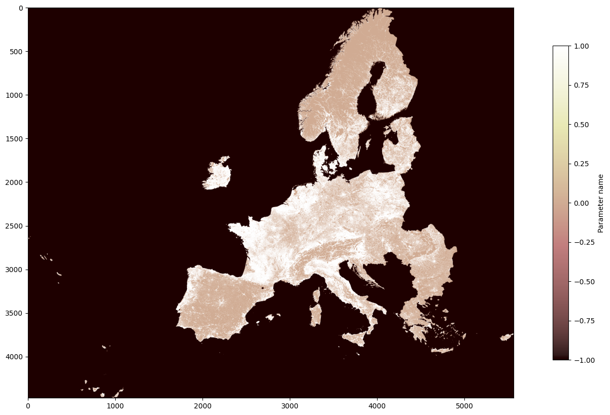
Plotting raster file#
There are couple of options to plot raster file. Below we present most popular option using matplotlib.pyplot module and tool implemented in rasterio package. More information:
https://matplotlib.org/3.5.3/api/_as_gen/matplotlib.pyplot.html
https://rasterio.readthedocs.io/en/stable/topics/plotting.html
# Plotting definition
fig, ax = pyplot.subplots(1, figsize=(20,10))

# Plotting raster
pyplot.imshow(raster_data[0], cmap='pink')

# Plotting color bar
pyplot.colorbar(label='Parameter name', fraction=0.02, ax=ax)
<matplotlib.colorbar.Colorbar at 0x7f63603d8f40>
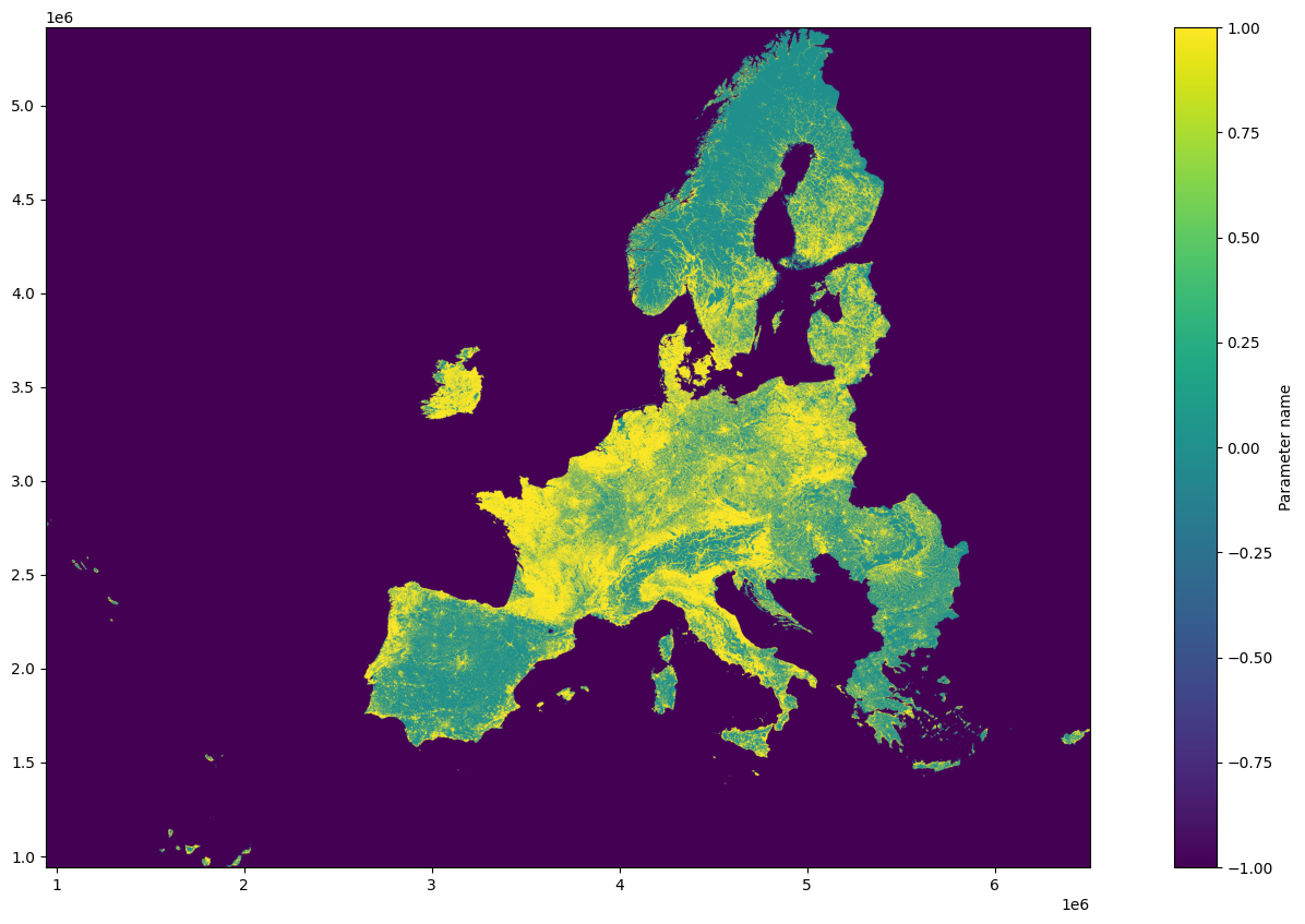
# Rasterio also provides rasterio.plot.show() to perform common tasks such as displaying
# multi-band images as RGB and labeling the axes with proper geo-referenced extents.

# Plotting definition
fig, ax = pyplot.subplots(1, figsize=(20,10))

# Plotting raster with georeference
rs = show(raster_data[0], ax=ax, transform=src.transform)

# Plotting color bar
fig.colorbar(rs.get_images()[0], ax=ax, label='Parameter name')
<matplotlib.colorbar.Colorbar at 0x7f63620b2e30>
Reading Parquet file to GeoDataFrame#
%%time

object_path = 'Census_GRID/2021/ESTAT_Census_2021_V2.parquet'

# Create a temporary directory to store parquet file
with tempfile.TemporaryDirectory() as tmpdirname:
    # Define local path to save parquet
    local_parquet_path = os.path.join(tmpdirname, object_path.split('/')[-1])

    # Download the parquet file from S3
    s3.download_file('ESTAT', object_path, local_parquet_path)

    # Read the parquet into a GeoDataFrame
    gdf = gpd.read_parquet(local_parquet_path)
CPU times: user 6.18 s, sys: 2.2 s, total: 8.38 s
Wall time: 7.42 s
gdf.info()
<class 'geopandas.geodataframe.GeoDataFrame'>
RangeIndex: 4594018 entries, 0 to 4594017
Data columns (total 18 columns):
 #   Column              Dtype
---  ------              -----
 0   GRD_ID              object
 1   T                   int64
 2   M                   float64
 3   F                   float64
 4   Y_LT15              float64
 5   Y_1564              float64
 6   Y_GE65              float64
 7   EMP                 float64
 8   NAT                 float64
 9   EU_OTH              float64
 10  OTH                 float64
 11  SAME                float64
 12  CHG_IN              float64
 13  CHG_OUT             float64
 14  LAND_SURFACE        float64
 15  POPULATED           int64
 16  CONFIDENTIALSTATUS  float64
 17  geom                geometry
dtypes: float64(14), geometry(1), int64(2), object(1)
memory usage: 630.9+ MB
gdf_filter.info()
<class 'geopandas.geodataframe.GeoDataFrame'>
RangeIndex: 101 entries, 0 to 100
Data columns (total 18 columns):
 #   Column              Non-Null Count  Dtype
---  ------              --------------  -----
 0   GRD_ID              101 non-null    object
 1   T                   101 non-null    int64
 2   M                   101 non-null    float64
 3   F                   101 non-null    float64
 4   Y_LT15              101 non-null    float64
 5   Y_1564              101 non-null    float64
 6   Y_GE65              101 non-null    float64
 7   EMP                 101 non-null    float64
 8   NAT                 101 non-null    float64
 9   EU_OTH              101 non-null    float64
 10  OTH                 101 non-null    float64
 11  SAME                101 non-null    float64
 12  CHG_IN              101 non-null    float64
 13  CHG_OUT             101 non-null    float64
 14  LAND_SURFACE        101 non-null    float64
 15  POPULATED           101 non-null    int64
 16  CONFIDENTIALSTATUS  0 non-null      float64
 17  geometry            101 non-null    geometry
dtypes: float64(14), geometry(1), int64(2), object(1)
memory usage: 14.3+ KB
Writing back data to the Read-Write S3 bucket#
from botocore.config import Config

custom_config = Config(
   request_checksum_calculation='WHEN_REQUIRED',
   response_checksum_validation='WHEN_REQUIRED'
)

s3_client = boto3.client('s3', endpoint_url=credentials['host_base'],
                      aws_access_key_id=credentials['access_key'],
                      aws_secret_access_key=credentials['secret_key'],
                      use_ssl=True,
                      verify=False,
                      config=custom_config)

response = s3_client.list_buckets()
print(response['Buckets'])
[{'Name': 'estat-test', 'CreationDate': datetime.datetime(2025, 3, 4, 14, 28, 54, 502000, tzinfo=tzlocal())}]
from io import BytesIO

# Convert the GeoDataFrame to a Parquet file in-memory
buffer = BytesIO()
gdf_filter.to_parquet(buffer, engine='pyarrow')
buffer.seek(0)  # Move to the beginning of the buffer

# Specify your S3 bucket and file name
bucket_name = response['Buckets'][0]['Name']
file_name = 'teszt.parquet'

# Upload the file
s3_client.upload_fileobj(buffer, bucket_name, file_name)
response = s3.list_objects_v2(Bucket=bucket_name)
if 'Contents' in response:
    print("Objects in bucket:")
    # Iterate over each object
    for obj in response['Contents']:
        print(obj['Key'])
else:
    print("No objects found in the bucket.")
Objects in bucket:
teszt.parquet